import numpy as np
import matplotlib.pyplot as plt
from scipy.optimize import curve_fit
import pandas as pd
import statsmodels.api as sm
Take a look at these models \[ \begin{aligned} &Y_{i}=\beta_{1}+\beta_{2}\left(\frac{1}{X_{i}}\right)+u_{i}\\ &Y_{i}=\beta_{1}+\beta_{2} \ln X_{i}+u_{i}\\ &\text { In } Y_{i}=\beta_{1}+\beta_{2} X_{i}+u_{i}\\ &\ln Y_{i}=\ln \beta_{1}+\beta_{2} \ln X_{i}+u_{i}\\ &\ln Y_{i}=\beta_{1}-\beta_{2}\left(\frac{1}{X_{i}}\right)+u_{i} \end{aligned} \] The variables might have some nonlinear form, but parameters are all linear (the \(4\)th model can denote \(\alpha_1=\ln{\beta_1}\)), as long as we can convert them into linear form with some mathematical manipulation, we call them intrinsically linear models.
How about these two models? \[\begin{aligned} &Y_{i}=e^{\beta_{1}+\beta_{2} X_{i}+u_{i}} \\ &Y_{i}=\frac{1}{1+e^{\beta_{1}+\beta_{2} X_{i}+u_{i}}} \\ \end{aligned}\]The first one can be easily converted into linear one by taking natural log \[ \ln{Y_i}=\beta_{1}+\beta_{2} X_{i}+u_{i} \] The second one is bit tricky, we will deal with it in more details in chapter of binary choice model. But you can be assured that with a little manipulation the model becomes \[ \ln \left(\frac{1-Y_{i}}{Y_{i}}\right)=\beta_{1}+\beta_{2} X_{i}+u_{i} \] which is also intrinsically linear.
These two models are intrinsically nonlinear model, there is no way to turn them into linear form. \[\begin{aligned} &Y_{i}=\beta_{1}+\left(0.75-\beta_{1}\right) e^{-\beta_{2}\left(X_{i}-2\right)}+u_{i} \\ &Y_{i}=\beta_{1}+\beta_{2}^{3} X_{i}+u_{i}\\ \end{aligned}\] Can we transform Cobb-Douglas model into linear form? The first one can, by taking natural log. But the second one has an additive disturbance term, which make it intrinsically nonlinear. \[\begin{aligned} &Y_{i}=\beta_{1} X_{2 i}^{\beta_{2}} X_{3 i}^{\beta_{3}} u_{i}\\ &Y_{i}=\beta_{1} X_{2 i}^{\beta_{2}} X_{3 i}^{\beta_{3}}+ u_{i}\\ \end{aligned}\]Here is another famous economic model, constant elasticity of substitution (CES) production function. \[ Y_{i}=A\left[\delta K_{i}^{-\beta}+(1-\delta) L_{i}^{-\beta}\right]^{-1 / \beta}u_i \] No matter what you do with it, it can’t be transformed into linear form, thus it is intrinsically nonlinear
OLS On A Nonlinear Model
Consider an intrinsically nonlinear model \[ Y_{i}=\beta_{1} e^{\beta_{2}X_{i}}+u_{i} \] Use the OLS algorithm that minimize \(RSS\) \[ \begin{gathered} \sum_{i=0}^n u_{i}^{2}=\sum_{i=0}^n\left(Y_{i}-\beta_{1} e^{\beta_{2} X_{i}}\right)^{2} \end{gathered} \] Take partial derivative with respect to both \(\beta_1\) and \(\beta_2\), the first order conditions are \[ \begin{gathered} \frac{\partial \sum_{i=0}^n u_{i}^{2}}{\partial \beta_{1}}=2 \sum_{i=0}^n\left(Y_{i}-\beta_{1} e^{\beta_{2} X_{i}}\right)\left(-1 e^{\beta_{2} X_{i}}\right) =0\\ \frac{\partial \sum_{i=0}^n u_{i}^{2}}{\partial \beta_{2}}=2 \sum_{i=0}^n\left(Y_{i}-\beta_{1} e^{\beta_{2} X_{i}}\right)\left(-\beta_{1} e^{\beta_{2} X_{i}} X_{i}\right)=0 \end{gathered} \]
Collecting terms and denote the estimated coefficients as \(b_1\) and \(b_2\) \[ \begin{aligned} \sum_{i=0}^n Y_{i} e^{b_{2} X_{i}} &=b_{1} e^{2 {b}_{2} X_{i}} \\ \sum_{i=0}^n Y_{i} X_{i} e^{b_{2} X_{i}} &={b}_{1} \sum_{i=0}^n X_{i} e^{2 {b}_{2} X_{i}} \end{aligned} \]
These are solutions, but not closed-form solution, i.e. solve by plugging in data. So even if you have these formula, we can’t input in Python, because unknowns are expressed in terms of unknowns.
Gauss-Newton Iterative Method
We will not talk about details of this algorithm, it only confuses you more than clarification. But this Gauss-Newton Iterative Method is kind of trial and error method that gradually approaching the optimized coefficients. It feeds the \(RSS\) formula with parameters, record the result, then try another set of parameters, if \(RSS\) gets smaller, the algorithm keeps feed parameters until the \(RSS\) have no significant improvement.
Define the function \[ Y_{i}=\beta_{1} e^{\beta_{2}X_{i}} \]
def exp_func(x, beta1, beta2):
    return beta1 * np.exp(beta2 * x)
Simulate data \(Y\) then estimate the parameters with curve_fit function
xdata = np.linspace(0, 1, 50)
y = exp_func(xdata, 2, 3)

y_noise = 5 * np.random.randn(len(y))
ydata = y + y_noise
fig, ax = plt.subplots(figsize=(12, 8))
ax.scatter(xdata, ydata, label="data", color="purple")
popt, pcov = curve_fit(exp_func, xdata, ydata)
ax.plot(xdata, exp_func(xdata, popt[0], popt[1]), lw=3, color="tomato")
ax.set_title(r"$Y_{i}=\beta_{1} e^{\beta_{2}X_{i}}$")
plt.show()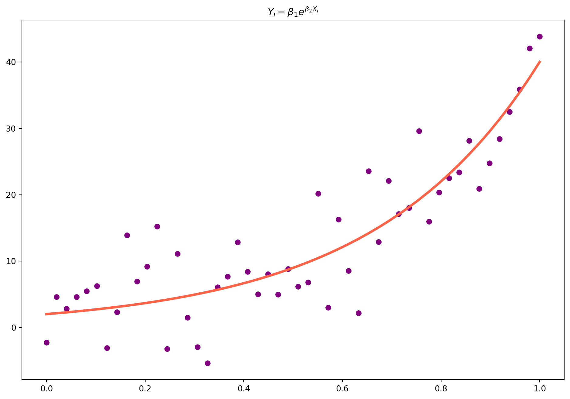
Given the fact that this is elementary course on econometrics, we will not go any deeper in this topic. In Advanced Econometrics, we will have a very extensive discussion of nonlinear regression.
Shanghai Covid
df_shcovid = pd.read_excel("../dataset/shanghai_covid_stats.xlsx")df_shcovid.columns = ["Date", "Cases"]
df_shcovid = df_shcovid.dropna()Define the function \[ Y_{i}= \beta_1 e^{\beta_{2}X_{i}} \]
Take log on both sides. \[ \ln{Y_i}=\ln{\beta_1}+\beta_2 X_i \]
logY = np.log(df_shcovid["Cases"])
X = np.arange(len(logY))

X = sm.add_constant(X)
model = sm.OLS(logY, X).fit()

print_model = model.summary()
print(print_model)
OLS Regression Results
==============================================================================
Dep. Variable: Cases R-squared: 0.959
Model: OLS Adj. R-squared: 0.957
Method: Least Squares F-statistic: 463.3
Date: Sun, 27 Oct 2024 Prob (F-statistic): 2.65e-15
Time: 17:35:47 Log-Likelihood: -3.9519
No. Observations: 22 AIC: 11.90
Df Residuals: 20 BIC: 14.09
Df Model: 1
Covariance Type: nonrobust
==============================================================================
coef std err t P>|t| [0.025 0.975]
------------------------------------------------------------------------------
const 5.4038 0.125 43.157 0.000 5.143 5.665
x1 0.2197 0.010 21.524 0.000 0.198 0.241
==============================================================================
Omnibus: 3.277 Durbin-Watson: 0.593
Prob(Omnibus): 0.194 Jarque-Bera (JB): 1.649
Skew: -0.355 Prob(JB): 0.438
Kurtosis: 1.862 Cond. No. 23.8
==============================================================================
Notes:
[1] Standard Errors assume that the covariance matrix of the errors is correctly specified.beta_1 = np.exp(model.params.iloc[0])
beta_2 = model.params.iloc[1]
Y = beta_1 * np.exp(beta_2 * X[:, 1])fig, ax = plt.subplots(figsize=(12, 5), nrows=1, ncols=2)
fig.autofmt_xdate(rotation=45)
ax[0].scatter(df_shcovid["Date"], df_shcovid["Cases"])
ax[0].set_ylabel("No-Symptom Case")
ax[1].plot(df_shcovid["Date"], model.fittedvalues)
ax[0].plot(df_shcovid["Date"], Y)
ax[1].set_ylabel("Log No-Symptom Case")
ax[1].scatter(df_shcovid["Date"], np.log(df_shcovid["Cases"]))
plt.show()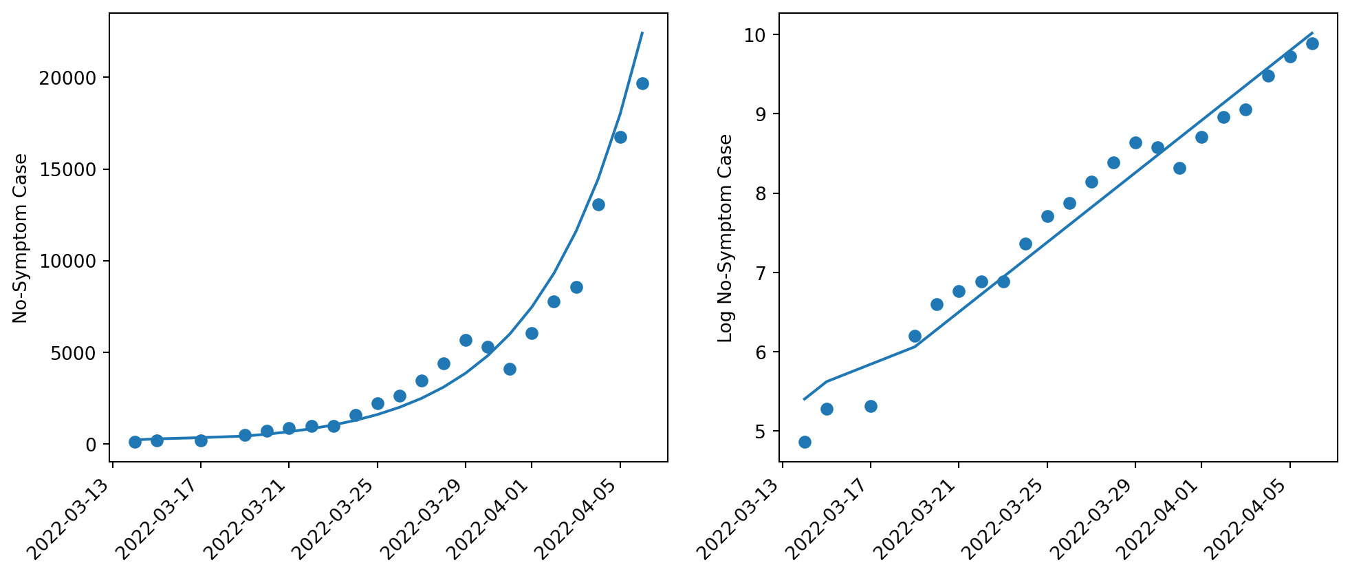
\[ Y_{i}= 5.4 e^{0.21X_{i}} \]